The cost-effectiveness of thermal comfort in the house is ensured by the calculation of hydraulics, its high-quality installation and proper operation. The main components of a heating system are a heat source (boiler), a heat main (pipes) and heat transfer devices (radiators). For effective heat supply, it is necessary to maintain the original parameters of the system under any load, regardless of the time of year. Before starting hydraulic calculations, perform:
- Collection and processing of information on the facility for the purpose of: determining the amount of heat required;
- choosing a heating scheme.
- volumes of thermal energy;
If water heating is considered the best option, a hydraulic calculation is performed.
Calculating hydraulics using programs requires familiarity with the theory and laws of resistance. If the formulas below seem difficult to understand, you can choose the parameters that we offer in each of the programs.
Calculations were carried out in Excel. The finished result can be seen at the end of the instructions.
What is hydraulic calculation
This is the third stage in the process of creating a heating network. It is a system of calculations that allows you to determine:
- pipe diameter and capacity;
- local pressure losses in areas;
- hydraulic linkage requirements;
- system-wide pressure losses;
- optimal water consumption.
According to the data obtained, pumps are selected.
For seasonal housing, in the absence of electricity, a heating system with natural coolant circulation is suitable (link to review).
The main goal of hydraulic calculation is to ensure that the calculated costs for the circuit elements match the actual (operating) costs. The amount of coolant entering the radiators must create a thermal balance inside the house, taking into account the external temperatures and those set by the user for each room according to its functional purpose (basement +5, bedroom +18, etc.).
Complex tasks - cost minimization:
- capital – installation of pipes of optimal diameter and quality;
- operational:
- dependence of energy consumption on the hydraulic resistance of the system;
- stability and reliability;
- noiselessness.
Replacing the centralized heat supply mode with an individual one simplifies the calculation method.
For the autonomous mode, 4 methods of hydraulic calculation of the heating system are applicable:
- by specific losses (standard calculation of pipe diameter);
- by lengths reduced to one equivalent;
- according to conductivity and resistance characteristics;
- comparison of dynamic pressures.
The first two methods are used with a constant temperature difference in the network.
The last two will help distribute hot water among the rings of the system if the temperature difference in the network no longer corresponds to the difference in the risers/branches.
Calculation of hydraulics of the heating system
We will need data from thermal calculations of the premises and an axonometric diagram.
Axonometric diagram
Enter your data into this table:
| No. of settlement area | Thermal load | Length |
| write down | write down | write down |
Step 1: count the diameter of the pipes
Economically justified results of thermal calculations are used as initial data:
1a. The optimal difference between hot (tg) and cooled (tо) coolant for a two-pipe system is 20º
- Δtco=tg- to=90º-70º=20ºС
1b. Coolant flow G, kg/hour - for a one-pipe system.
2. The optimal speed of coolant movement is ν 0.3-0.7 m/s.
The smaller the internal diameter of the pipes, the higher the speed. Reaching 0.6 m/s, the movement of water begins to be accompanied by noise in the system.
3. Design heat flow rate – Q, W.
Expresses the amount of heat (W, J) transferred per second (unit of time τ):
Formula for calculating heat flow rate
4. Estimated density of water: ρ = 971.8 kg/m3 at tav = 80 °C
5. Parameters of sections:
| Plot | Section length, m | Number of devices N, pcs |
| 1 — 2 | 1.78 | 1 |
| 2 — 3 | 2.60 | 1 |
| 3 — 4 | 2.80 | 2 |
| 4 — 5 | 2.80 | 2 |
| 5 — 6 | 2.80 | 4 |
| 6 — 7 | 2.80 | |
| 7 — 8 | 2.20 | |
| 8 — 9 | 6.10 | 1 |
| 9 — 10 | 0.5 | 1 |
| 10 — 11 | 0.5 | 1 |
| 11 — 12 | 0.2 | 1 |
| 12 — 13 | 0.1 | 1 |
| 13 — 14 | 0.3 | 1 |
| 14 — 15 | 1.00 | 1 |
To determine the internal diameter for each section, it is convenient to use a table.
Explanation of abbreviations:
- dependence of the speed of water movement - ν, s
- heat flow - Q, W
- water consumption G, kg/hour from the internal diameter of the pipes
| Ø 8 | Ø 10 | Ø 12 | Ø 15 | Ø 20 | Ø 25 | Ø 50 | ||||||||||||||
| ν | Q | G | v | Q | G | v | Q | G | v | Q | G | v | Q | G | v | Q | G | v | Q | G |
| 0.3 | 1226 | 53 | 0.3 | 1916 | 82 | 0.3 | 2759 | 119 | 0.3 | 4311 | 185 | 0.3 | 7664 | 330 | 0.3 | 11975 | 515 | 0.3 | 47901 | 2060 |
| 0.4 | 1635 | 70 | 0.4 | 2555 | 110 | 0.4 | 3679 | 158 | 0.4 | 5748 | 247 | 0.4 | 10219 | 439 | 0.4 | 15967 | 687 | 0.4 | 63968 | 2746 |
| 0.5 | 2044 | 88 | 0.5 | 3193 | 137 | 0.5 | 4598 | 198 | 0.5 | 7185 | 309 | 0.5 | 12774 | 549 | 0.5 | 19959 | 858 | 0.5 | 79835 | 3433 |
| 0.6 | 2453 | 105 | 0.6 | 3832 | 165 | 0.6 | 5518 | 237 | 0.6 | 8622 | 371 | 0.6 | 15328 | 659 | 0.6 | 23950 | 1030 | 0.6 | 95802 | 4120 |
| 0.7 | 2861 | 123 | 0.7 | 4471 | 192 | 0.7 | 6438 | 277 | 0.7 | 10059 | 433 | 0.7 | 17883 | 769 | 0.7 | 27942 | 1207 | 0.7 | 111768 | 4806 |
Example
Task : select the diameter of the pipe for heating a living room with an area of 18 m², ceiling height 2.7 m.
Project data:
- two-pipe wiring diagram;
- circulation is forced (pump).
Average data:
- power consumption – 1 kW per 30 m³
- thermal power reserve – 20%
Calculation:
- room volume: 18 * 2.7 = 48.6 m³
- power consumption: 48.6 / 30 = 1.62 kW
- reserve in case of frost: 1.62 * 20% = 0.324 kW
- total power: 1.62 + 0.324 = 1.944 kW
We find the closest Q value in the table:
We get the interval of internal diameter: 8-10 mm. Section: 3-4. Section length: 2.8 meters.
Step 2: Calculate Local Resistances
To decide on the pipe material, it is necessary to compare the indicators of their hydraulic resistance in all areas of the heating system.
Factors of resistance:
Heating pipes
- in the pipe itself: roughness;
- place of narrowing/expansion of diameter;
- turn;
- length.
- tee;
The design section is a pipe of constant diameter with a constant water flow corresponding to the design heat balance of the room.
To determine losses, data is taken taking into account the resistance in the control valves:
- pipe length at the design section/l, m;
- pipe diameter of the calculated section/d, mm;
- accepted coolant speed/u, m/s;
- control valve data from the manufacturer;
- reference data:
- friction coefficient/λ;
- friction losses/∆Рl, Pa;
- calculated liquid density/ρ = 971.8 kg/m3;
- Product specifications:
- equivalent pipe roughness/ke mm;
- pipe wall thickness/dн×δ, mm.
For materials with similar ke values, manufacturers provide the value of specific pressure loss R, Pa/m for the entire range of pipes.
To independently determine the specific friction losses/R, Pa/m, it is enough to know the outer d of the pipe, the wall thickness/dн×δ, mm and the water supply speed/W, m/s (or water flow/G, kg/h).
To search for hydraulic resistance/ΔP in one section of the network, we substitute the data into the Darcy-Weisbach formula: For steel and polymer pipes (made of polypropylene, polyethylene, fiberglass, etc.), the friction coefficient/λ is most accurately calculated using the Altschul formula: Re - Reynolds number , is found using a simplified formula (Re=v*d/ν) or using an online calculator:
Step 3: hydraulic linkage
To balance pressure differences, you will need shut-off and control valves.
Initial data:
- design load (mass flow of coolant - water or low-freezing liquid for heating systems);
- data from pipe manufacturers on specific dynamic resistance/A, Pa/(kg/h)²;
- technical characteristics of fittings.
- the number of local resistances in the area.
Task : to equalize hydraulic losses in the network.
In the hydraulic calculation, installation characteristics (mounting, pressure drop, flow capacity) are specified for each valve. Based on the resistance characteristics, the coefficients of flow into each riser and then into each device are determined.
Fragment of factory characteristics of a butterfly valve
Let us choose for calculations the method of resistance characteristics S, Pa/(kg/h)².
Pressure loss/∆P, Pa is directly proportional to the square of water flow over the area/G, kg/h: In the physical sense, S is the pressure loss per 1 kg/h of coolant: where:
- ξpr - reduced coefficient for local resistances of the section;
- A - dynamic specific pressure, Pa/(kg/h)².
The specific pressure is considered to be the dynamic pressure that occurs at a mass flow rate of 1 kg/h of coolant in a pipe of a given diameter (information provided by the manufacturer).
Σξ is the term of the coefficients for local resistance in the section.
Reduced coefficient: It sums up all local resistance: With a value: which corresponds to the coefficient of local resistance taking into account losses from hydraulic friction.
Step 4: Determine losses
The hydraulic resistance in the main circulation ring is represented by the sum of the losses of its elements:
- primary circuit/ΔPIк ;
- local systems/ΔPm;
- heat generator/ΔPtg;
- heat exchanger/ΔPto.
The sum of the values gives us the hydraulic resistance of the system/ΔPco:
Calculation of local resistances
Local resistances arise in the pipe and fittings. The value of these indicators is influenced by:
- roughness of the inner surface of the pipe;
- the presence of areas of expansion or contraction of the internal diameter of the pipeline;
- turns;
- length;
- the presence of tees, ball valves, balancing devices and their number.
The resistance is calculated for each section, which is characterized by a constant diameter and constant coolant flow (in accordance with the heat balance of the room).
Initial data for calculation:
- length of the design section – l, m;
- pipe diameter – d, mm;
- specified coolant speed – u, mm;
- characteristics of control valves provided by the manufacturer;
- friction coefficient (depending on the pipe material), λ;
- friction losses – ∆Pl, Pa;
- coolant density (calculated) – ρ = 971.8 kg/m3;
- pipe wall thickness – dн x δ, mm;
- equivalent pipe roughness – ke, mm.
Hydraulic resistance - ∆P on a network section is calculated using the Darcy-Weisbach formula.
The symbol ξ in the formula means the local resistance coefficient.
Program overview
For ease of calculations, amateur and professional hydraulic calculation programs are used.
The most popular is Excel.
You can use online calculation in Excel Online, CombiMix 1.0, or online hydraulic calculation calculator. The stationary program is selected taking into account the requirements of the project.
The main difficulty in working with such programs is ignorance of the basics of hydraulics. Some of them lack explanations of formulas, and do not consider the features of branching pipelines and calculating resistance in complex circuits.
Features of the programs:
- HERZ CO 3.5 – performs calculations using the specific linear pressure loss method.
- DanfossCO and OvertopCO - can count systems with natural circulation.
- “Flow” (Potok) - allows you to use a calculation method with a variable (sliding) temperature difference along the risers.
It is necessary to clarify the parameters for entering temperature data - in Kelvin/Celsius.
How to work in EXCEL
Using Excel tables is very convenient, since the results of hydraulic calculations are always reduced to tabular form. It is enough to determine the sequence of actions and prepare exact formulas.
Entering initial data
Select a cell and enter a value. All other information is simply taken into account.
| Cell | Magnitude | Meaning, designation, unit of expression |
| D4 | 45,000 | Water consumption G in t/hour |
| D5 | 95,0 | Inlet temperature tin in °C |
| D6 | 70,0 | Outlet temperature tout in °C |
| D7 | 100,0 | Inner diameter d, mm |
| D8 | 100,000 | Length, L in m |
| D9 | 1,000 | Equivalent pipe roughness ∆ in mm |
| D10 | 1,89 | Sum coefficient local resistance - Σ(ξ) |
Explanations:
- the value in D9 is taken from the directory;
- the value in D10 characterizes the resistance at the welds.
Formulas and algorithms
We select cells and enter the algorithm, as well as the formulas of theoretical hydraulics.
| Cell | Algorithm | Formula | Result | Result value |
| D12 | !ERROR! D5 does not contain a number or expression | tср=(tin+tout)/2 | 82,5 | Average water temperature tav in °C |
| D13 | !ERROR! D12 does not contain a number or expression | n=0.0178/(1+0.0337*tavg+0.000221*tavg2) | 0,003368 | Kinematic coefficient water viscosity - n, cm2/s at tav |
| D14 | !ERROR! D12 does not contain a number or expression | ρ=(-0.003*tav2-0.1511*tav+1003, 1)/1000 | 0,970 | Average water density ρ,t/m3 at tav |
| D15 | !ERROR! D4 does not contain a number or expression | G'=G*1000/(ρ*60) | 773,024 | Water consumption G', l/min |
| D16 | !ERROR! D4 does not contain a number or expression | v=4*G:(ρ*π*(d:1000)2*3600) | 1,640 | Water speed v, m/s |
| D17 | !ERROR! D16 does not contain a number or expression | Re=v*d*10/n | 487001,4 | Reynolds number Re |
| D18 | !ERROR! Cell D17 does not exist | λ=64/Re at Re≤2320 λ=0.0000147*Re at 2320≤Re≤4000 λ=0.11*(68/Re+∆/d)0.25 at Re≥4000 | 0,035 | Hydraulic friction coefficient λ |
| D19 | !ERROR! Cell D18 does not exist | R=λ*v2*ρ*100/(2*9.81*d) | 0,004645 | Specific friction pressure loss R, kg/(cm2*m) |
| D20 | !ERROR! Cell D19 does not exist | dPtr=R*L | 0,464485 | Friction pressure loss dPtr, kg/cm2 |
| D21 | !ERROR! Cell D20 does not exist | dPtr=dPtr*9.81*10000 | 45565,9 | and Pa respectively D20 |
| D22 | !ERROR! D10 does not contain a number or expression | dPms=Σ(ξ)*v2*ρ/(2*9.81*10) | 0,025150 | Pressure loss in local resistance dPms in kg/cm2 |
| D23 | !ERROR! Cell D22 does not exist | dPtr=dPms*9.81*10000 | 2467,2 | and Pa respectively D22 |
| D24 | !ERROR! Cell D20 does not exist | dP=dPtr+dPms | 0,489634 | Calculated pressure loss dP, kg/cm2 |
| D25 | !ERROR! Cell D24 does not exist | dP=dP*9.81*10000 | 48033,1 | and Pa respectively D24 |
| D26 | !ERROR! Cell D25 does not exist | S=dP/G2 | 23,720 | Resistance characteristic S, Pa/(t/h)2 |
Explanations:
- the D15 value is recalculated in liters, this makes it easier to perceive the flow rate;
- cell D16 - add formatting according to the condition: “If v does not fall within the range of 0.25...1.5 m/s, then the cell background is red/the font is white.”
For pipelines with a difference in inlet and outlet heights, static pressure is added to the results: 1 kg/cm2 per 10 m.
Registration of results
The author's color scheme carries a functional load:
- Light turquoise cells contain the original data - they can be changed.
- Pale green cells are entered constants or data that is little subject to change.
- Yellow cells are auxiliary preliminary calculations.
- Light yellow cells—calculation results.
- Fonts: blue - original data;
- black - intermediate/non-main results;
- red - the main and final results of the hydraulic calculation.
Results in Excel table
Example from Alexander Vorobyov
An example of a simple hydraulic calculation in Excel for a horizontal pipeline section.
Initial data:
- pipe length 100 meters;
- ø108 mm;
- wall thickness 4 mm.
Table of results for calculating local resistances
By complicating the calculations in Excel step by step, you better master the theory and partially save on design work. Thanks to a competent approach, your heating system will become optimal in terms of costs and heat transfer.
Pipe diameter calculation
Calculation of pipe cross-sections should be based on the results of thermal calculations that are economically justified:
- for a two-pipe system - the difference between tr (hot coolant) and to (cooled - return);
- for single-pipe – coolant flow G, kg/h.
In addition, the calculation must take into account the speed of movement of the working fluid (coolant) - V. Its optimal value is in the range of 0.3-0.7 m/s. The speed is inversely proportional to the internal diameter of the pipe.
When the water speed is 0.6 m/s, characteristic noise appears in the system, but if it is less than 0.2 m/s, there is a risk of air jams.
For calculations, one more speed characteristic will be required - the heat flow rate. It is designated by the letter Q, measured in watts and expressed as the amount of heat transferred per unit time
Q (W) = W (J)/t (s)
In addition to the above initial data, the calculation will require the parameters of the heating system - the length of each section, indicating the devices connected to it. For convenience, these data can be summarized in a table, an example of which is given below.
Table of plot parameters
| Site designation | Section length in meters | Number of devices in the area, pcs. |
| 1-2 | 1,8 | 1 |
| 2-3 | 3,0 | 1 |
| 3-4 | 2,8 | 2 |
| 4-5 | 2,9 | 2 |
Calculating pipe diameters is quite complex, so it’s easier to use reference tables. They can be found on the websites of pipe manufacturers, in SNiP or specialized literature.
When selecting pipe diameters, installers use a rule derived from an analysis of a large number of heating systems. True, this only applies to small private houses and apartments. Almost all heating boilers are equipped with ¾ and ½ inch supply and return pipes. This pipe is used for wiring up to the first branch. Next, at each section, the pipe size is reduced by one step.
This approach does not justify itself if the house has two or more floors. In this case, you have to make a full calculation and refer to the tables.